4.2. Thermal Examples
Structural Fire Engineering
The following types of fire analyses are represented in these examples. The fire analysis is performed is a stress-based analysis where the temperature of the elements is set within the code. Heat transfer analysis between the gas temperatures and the structural member should be performed using lump mass heat transfer analysis techniques or appropriate finite element programs.
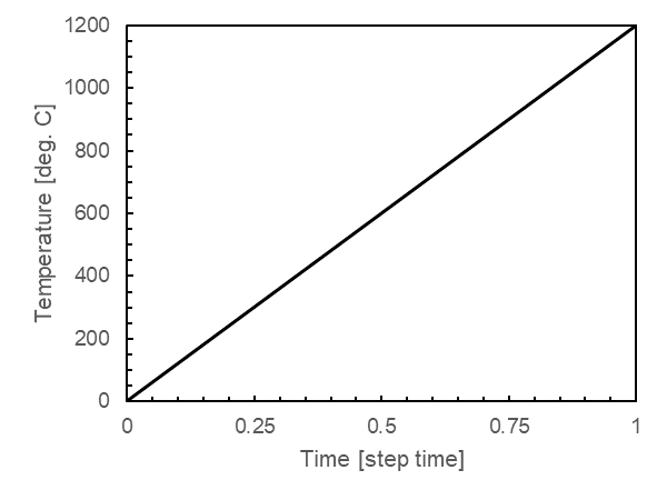
4.2.6. Target temperature
The temperature of the elements are set and a linear time-temperature curve is assumed for each element to reach the set temperature over the time period of the step.

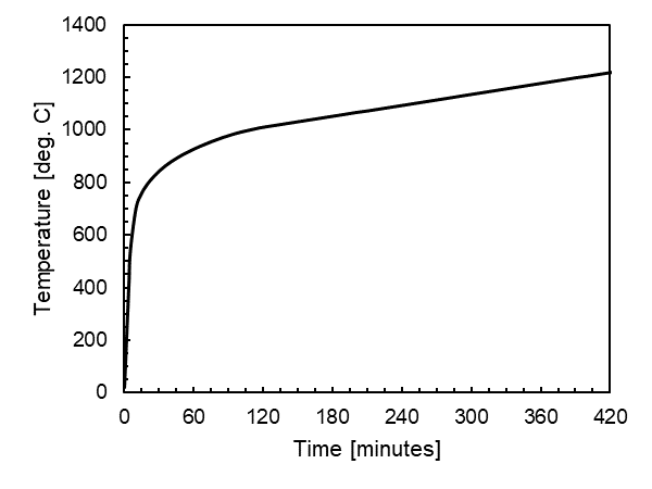
4.2.7. Standard fire curve
The standard fire curve is defined by ASTM E119 and ISO 834. These two curves are essentially the same and are used for standardized fire testing. These time-temperature curves increase rapidly at the beginning and then steadily increase over a time period of eight hours.

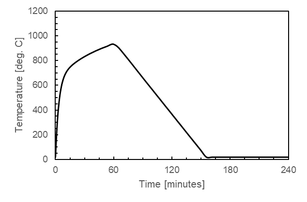
4.2.8. Parametric time-temperature fire curve
When the research involves structural fire engineering, a parametric time-temperature curve that is based on Eurocode 1 may be required. This time-temperature curve is dependent upon the ventilation (openings) in the compartment, the material of the compartment, the fuel load density, and the size of the compartment. These factors combined will produce a time-temperature curve that characterizes the fire in the compartment under consideration. The shape of this curve and the maximum temperature is highly dependent upon all of the factors previously listed. This type of fire curve will also include a cooling portion of the fire, when all of the fuel has been consumed. This type of fire time-temperature curve is used when a complete burn out fire scenario is being investigated.

4.2.9. Simulation process
Each example script does the following:
Build the model
Model dimensions and degress-of-freedom
Nodal coordinates
Nodal constraints – boundary conditions
Nodal masses
Elements and element connectivity
Set element temperatures
Recorders for output
Define and apply gravity load
Nodal or element load
Static-analysis parameters (tolerances and load increments)
Analyze
Hold gravity loads constant
Reset time to zero
Define and apply element temperatures
Load pattern (nodal loads for gravity analysis and temperature patterns for fire)
Provide temperature history for the loads either through a set temperature or reference to a time-temperature curve
Analyze