MIMO for a Ground Motion Event#

Chopra Section 9.7#

Partitioned equation of dynamic equilibrium (Chopra Eq. 9.7.1)#

\[\begin{split}\begin{bmatrix} \mathbf{m} & \mathbf{m}_g \\ \mathbf{m}^T_g & \mathbf{m}_{gg} \end{bmatrix} \begin{Bmatrix} \mathbf{\ddot{u}}^t \\ \mathbf{\ddot{u}}_g \end{Bmatrix} + \begin{bmatrix} \mathbf{c} & \mathbf{c}_g \\ \mathbf{c}^T_g & \mathbf{c}_{gg} \end{bmatrix} \begin{Bmatrix} \mathbf{\dot{u}}^t \\ \mathbf{\dot{u}}_g \end{Bmatrix} + \begin{bmatrix} \mathbf{k} & \mathbf{k}_g \\ \mathbf{k}^T_g & \mathbf{k}_{gg} \end{bmatrix} \begin{Bmatrix} \mathbf{u}^t \\ \mathbf{u}_g \end{Bmatrix} = \begin{Bmatrix} \mathbf{0} \\ \mathbf{p}_g(t) \end{Bmatrix}\end{split}\]

Problem Statement#

given: $\mathbf{u}_g$, $\mathbf{\dot{u}}_g$, and $\mathbf{\ddot{u}}_g$

find: $\mathbf{u}^t$ and $\mathbf{p}_g(t)$

–> (system ID: given output $\mathbf{u}^t$ and input $\mathbf{\ddot{u}}_g$, determine fundamental frequencies and mode shapes of the structure.)

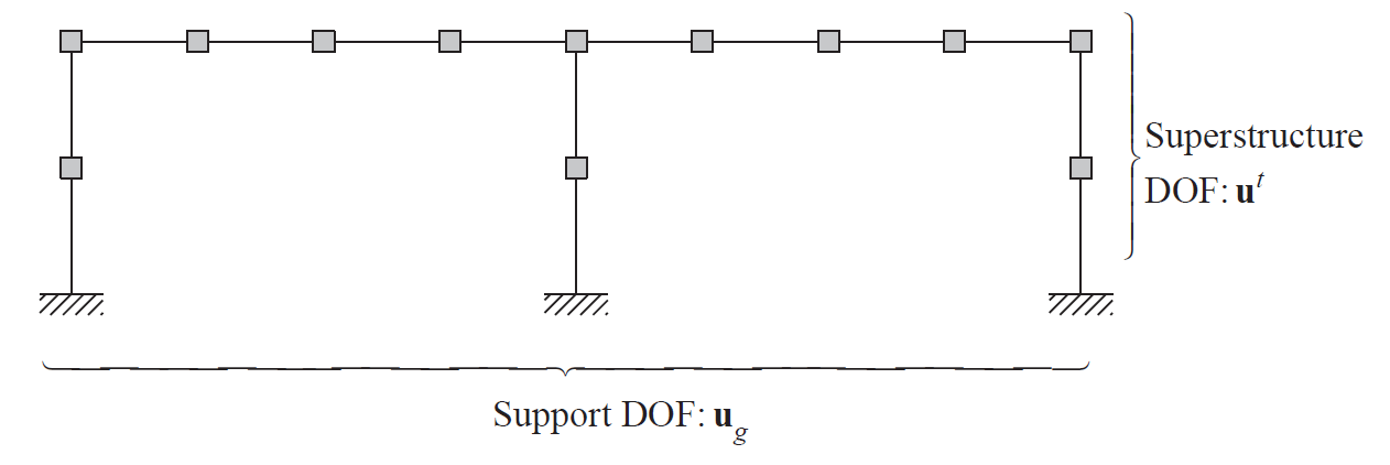
General equation of motion for multiple support excitation#

split displacements into quasi-static ($\mathbf{u}^s$) and dynamic ($\mathbf{u}$) displacements (chopra eq 9.7.2):

\[\begin{split}\begin{Bmatrix} \mathbf{u}^t \\ \mathbf{u}_g \end{Bmatrix} = \begin{Bmatrix} \mathbf{u}^s \\ \mathbf{u}_g \end{Bmatrix} + \begin{Bmatrix} \mathbf{u} \\ \mathbf{0} \end{Bmatrix}\end{split}\]

take the first half of the partitioned equilibrium equation from eq 9.7.1 (chopra eq 9.7.4)

\[\mathbf{m}\mathbf{\ddot{u}}^t + \mathbf{m}_g\mathbf{\ddot{u}}_g + \mathbf{c}\mathbf{\dot{u}}^t + \mathbf{c}_g\mathbf{\dot{u}}_g + \mathbf{k}\mathbf{u}^t + \mathbf{k}_g\mathbf{u}_g = \mathbf{0}\]

substitute eq 9.7.2 ($\mathbf{u}^t=\mathbf{u}^s+\mathbf{u}$) and move all $\mathbf{u}_g$ and $\mathbf{u}^s$ terms to the right side (chopra eq 9.7.5):

\[\mathbf{m}\mathbf{\ddot{u}} + \mathbf{c}\mathbf{\dot{u}} + \mathbf{k}\mathbf{u} = \mathbf{p}_{eff}(t)\]

where

\[\mathbf{p}_{eff}(t) = -(\mathbf{m}\mathbf{\ddot{u}}^s+\mathbf{m}_g\mathbf{\ddot{u}}_g) -(\mathbf{c}\mathbf{\dot{u}}^s+\mathbf{c}_g\mathbf{\dot{u}}_g) -(\mathbf{k}\mathbf{u}^s+\mathbf{k}_g\mathbf{u}_g)\]

which simplifies to

\[\mathbf{p}_{eff}(t) = -\mathbf{m}\mathbf{\iota}\mathbf{\ddot{u}}_g(t)\]
final equation of motion

\[\mathbf{m}\mathbf{\ddot{u}} + \mathbf{c}\mathbf{\dot{u}} + \mathbf{k}\mathbf{u} = -\mathbf{m}\mathbf{\iota}\mathbf{\ddot{u}}_g(t)\]

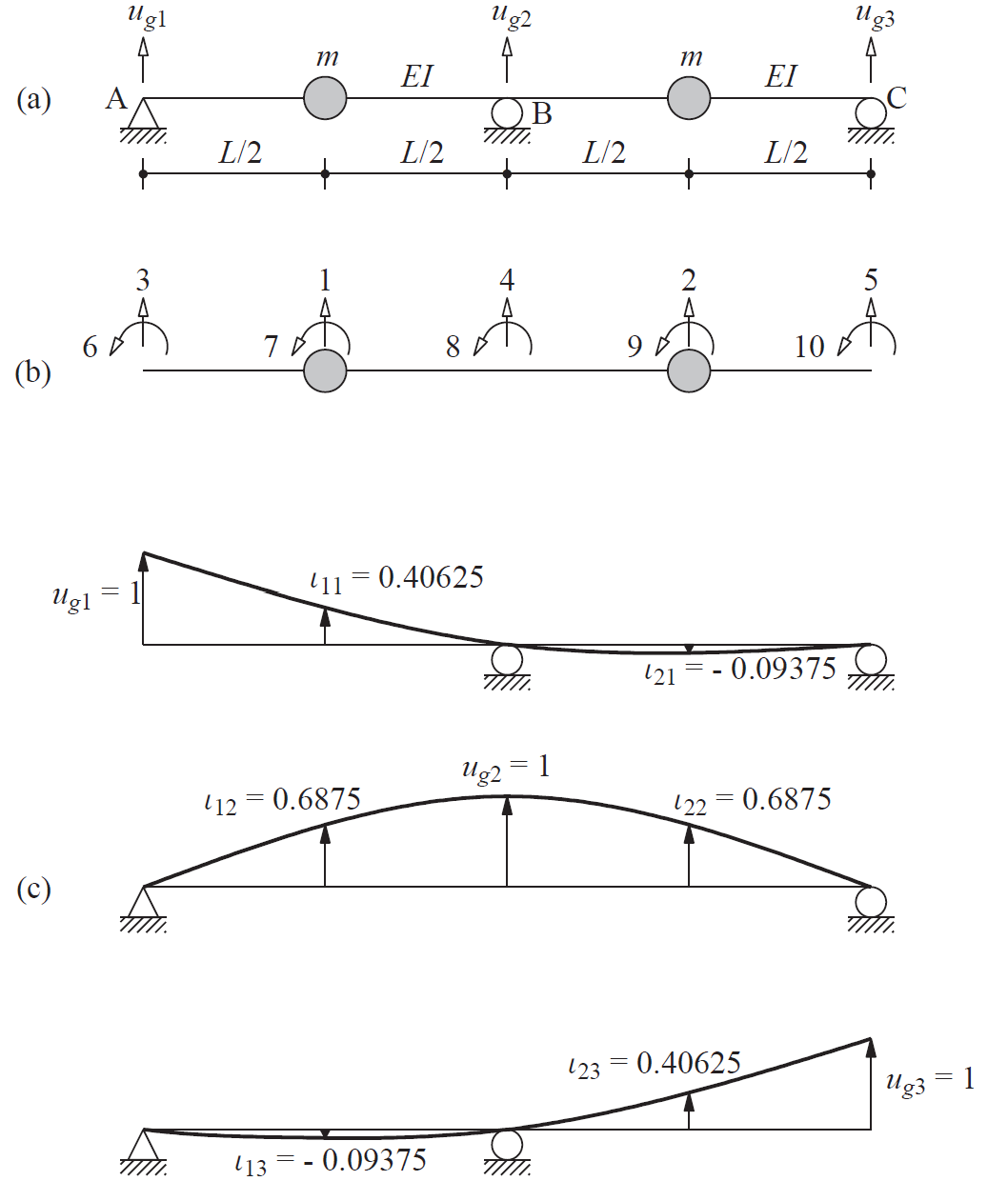
Example 9.10#

[1]:

import numpy as np
from matplotlib import pyplot as plt

# EI/L^3 = 1
EIL3 = 1
# m = 1
m_node = 1

k_hat = EIL3*np.array(
    [
        [78.86, 30.86, -29.14, -75.43, -5.14],
        [30.86, 78.86, -5.13, -75.43, -29.14],
        [-29.14, -5.14, 12.86, 20.57, 0.86],
        [-75.43, -75.43, 20.57, 109.71, 20.57],
        [-5.14, -29.14, 0.86, 20.57, 12.86]
    ]
)

k = k_hat[:2,:2]
k_g = k_hat[:2,2:]
k_gg = k_hat[2:,2:]

print(f"{k=}, \n{k_g=}, \n{k_gg=}")

m = m_node*np.identity(2)

print(f"{m=}")

iota = -np.linalg.inv(k)@k_g

print(f"{iota=}")

k=array([[78.86, 30.86],
       [30.86, 78.86]]),
k_g=array([[-29.14, -75.43,  -5.14],
       [ -5.13, -75.43, -29.14]]),
k_gg=array([[ 12.86,  20.57,   0.86],
       [ 20.57, 109.71,  20.57],
       [  0.86,  20.57,  12.86]])
m=array([[1., 0.],
       [0., 1.]])
iota=array([[ 0.40627442,  0.68747721, -0.09378418],
       [-0.09393392,  0.68747721,  0.40621582]])

Equation of motion for chopra example 9.10#

\[\mathbf{m}\mathbf{\ddot{u}} + \mathbf{k}\mathbf{u} = -\sum_{l=1}^{3}\mathbf{m}\mathbf{\iota}_l\mathbf{\ddot{u}}_{gl}(t)\]

where

\[\begin{split}m = m\begin{bmatrix} 1 & 0 \\ 0 & 1 \end{bmatrix}\end{split}\]

\[\begin{split}k = \frac{EI}{L^3}\begin{bmatrix} 78.86 & 30.86 \\ 30.86 & 78.86 \end{bmatrix}\end{split}\]

\[\begin{split}\iota_1 = \begin{Bmatrix}0.40625\\-0.09375\end{Bmatrix} \iota_2 = \begin{Bmatrix}0.68750\\0.68750\end{Bmatrix} \iota_1 = \begin{Bmatrix}-0.09375\\0.40625\end{Bmatrix}\end{split}\]

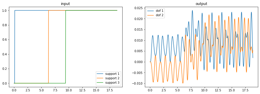
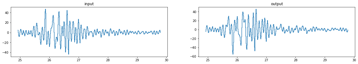
Plot example input and output motions for chopra example 9.10#

[2]:

from matplotlib import pyplot as plt
from scipy import integrate
from numpy import pi
tf = 6*pi
dt = 0.01
ns = 3
nf = 2
t = np.linspace(0., tf, 1000)
input = [
    lambda t: float(t > 0.1),
    lambda t: float(t > 2*pi),
    lambda t: float(t > 3*pi)
    # lambda t: np.sin(t),
    # lambda t: np.sin(t),
    # lambda t: np.sin(t-0.1)
]
# input = np.sin(t) + 20*np.random.rand(nt)
fig, ax = plt.subplots(1,2, figsize=(15,5))
ax[0].plot(t, [input[0](ti) for ti in t], t, [input[1](ti) for ti in t], t, [input[2](ti) for ti in t])
ax[0].set_title('input')
ax[0].legend(["support 1", "support 2", "support 3"])
minvk = np.linalg.inv(m)@k
def ex910(y,t,minvk,iota):
    dydt = y
    mipeff = sum(input[i](t)*iota[:,i] for i in range(ns))
    return np.array([
        *y[nf:],
        *(mipeff - minvk@y[:nf])
    ])
output = integrate.odeint(ex910, np.zeros(4), t, args=(minvk,iota))
ax[1].plot(t, output[:,0], t, output[:,1])
ax[1].set_title('output')
ax[1].legend(["dof 1", "dof 2"]);

../_images/examples_05_MIMO_Event_8_0.png

[3]:

import scipy
D, V = scipy.linalg.eig(k, m)
print(f"{V=}, \n{D=}")
D, V = np.linalg.eig(minvk)
print(f"{V=}, \n{D=}")
freqs = D**0.5
print(f"{freqs=}")

V=array([[-0.70710678, -0.70710678],
       [ 0.70710678, -0.70710678]]),
D=array([ 48.  +0.j, 109.72+0.j])
V=array([[ 0.70710678, -0.70710678],
       [ 0.70710678,  0.70710678]]),
D=array([109.72,  48.  ])
freqs=array([10.4747315 ,  6.92820323])

The fundamental frequencies of the system are 10.47 rad/s and 6.93 rad/s.

☐ get fundamental frequencies and mode shapes from equation of motion
☐ use system identification to determine fundamental frequencies and mode shapes

[4]:

t[1]

[4]:

0.018868424345884642

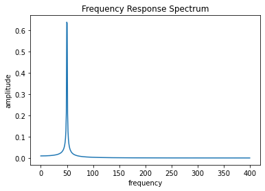
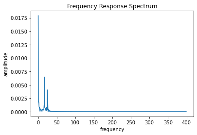
[5]:

from scipy.fft import fft, fftfreq
N = 1000
# T = t[1]
# T = 0.0189
T = 1.0/800
x = np.linspace(0.0, N*T, N, endpoint=False)
y = np.sin(50.0*2.0*pi*x)
xf = fftfreq(N, T)[:N//2]
yf = fft(y)
yff = 2.0/N * np.abs(yf[0:N//2])
plt.plot(xf, yff)
plt.xlabel("frequency")
plt.ylabel("amplitude")
plt.title("Frequency Response Spectrum")
freqs_fft = xf[np.argpartition(yff, -3)[-3:]]
print(f"{freqs_fft=}")

freqs_fft=array([48.8, 50.4, 49.6])

../_images/examples_05_MIMO_Event_13_1.png

[6]:

x = t
y = output[:,0]
N = len(x)
# T = x[1]
T = 1/800
xf = fftfreq(N,T)[:N//2]
yf = fft(y)
yff = 2.0/N * np.abs(yf[0:N//2])
plt.plot(xf, yff)
plt.xlabel("frequency")
plt.ylabel("amplitude")
plt.title("Frequency Response Spectrum")
# plt.xlim([0,5])
print([np.argpartition(yff, -5)[-5:]])
freqs_fft = xf[np.argpartition(yff, -5)[-5:]]
print(f"{freqs_fft=}")

[array([ 1, 21, 31, 32,  0], dtype=int64)]
freqs_fft=array([ 0.8, 16.8, 24.8, 25.6,  0. ])

../_images/examples_05_MIMO_Event_14_1.png

[7]:

print(f"{freqs[1]/freqs[0]=}")
print(f"{freqs_fft[1]/freqs_fft[0]=}")

freqs[1]/freqs[0]=0.6614206034955363
freqs_fft[1]/freqs_fft[0]=21.0

[8]:

freqs_fft[:2]/freqs/pi

# np.sqrt(2)/2
np.sqrt(3)/2

[8]:

0.8660254037844386

Parameterization of inputs and outputs for OKID-ERA and SRIM#

I X O -> SS

Class SS - coeff: A, B, C, D - obsv: $\mathcal{O}_{p}$ or $V$ or $V_r$ - ctrl: $\mathcal{C}_{p}$ or $W$ or $W_s$ - shapes: $\Phi, \Psi$ - freq: $\Omega, \Lambda$

[9]:

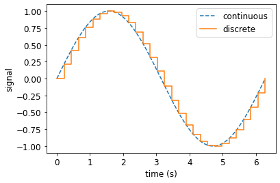
tf = 2*pi
t = np.linspace(0., tf, 1000)
td = np.linspace(0., tf, 30)

fig, ax = plt.subplots(figsize=(6,4))
ax.plot(t, np.sin(t), linestyle="--", label="continuous")
ax.step(td, np.sin(td), where='post', label="discrete")
ax.set_xlabel("time (s)", size=12)
ax.set_ylabel("signal", size=12)
ax.tick_params(axis='both', which='major', labelsize=12)
ax.legend(fontsize=12);

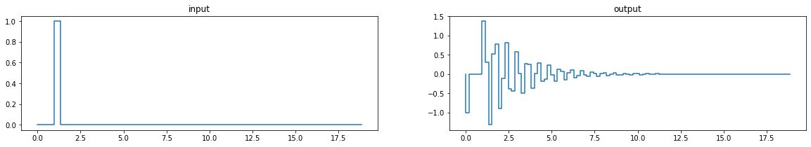
../_images/examples_05_MIMO_Event_18_0.png

[10]:

# SDOF example for impulse response and system id

# Timesteps
tf = 6*pi
nt = 100
t = np.linspace(0., tf, nt)
# Impulse input
input = lambda t: float(pi/3-0.1 < t < pi/3+0.1)

# Mass, stiffness, and damping
m = 1
k = 100
w = np.sqrt(k/m)
c = 0.05*2*m*w

fig, ax = plt.subplots(1,2, figsize=(20,3))
# fig, ax = plt.subplots(1,2, figsize=(10,3.5))
ax[0].step(t, [input(ti) for ti in t], where='post')
ax[0].set_title('input')
def eom(y,t,m,c,k):
    return [y[1], -k*y[0]/m-c*y[1]/m-input(t)]
output = integrate.odeint(eom, [1e-5,0], t, args=(m,c,k))
# ax[1].step(t, output[:,0], where='post')
# ax[1].plot(t, output[:,0], where='post')
ax[1].step(t, [-k*output[i,0]/m-c*output[i,1]/m-input(i) for i in range(nt)])
# ax[1].plot(t, [-k*output[i,0]/m-c*output[i,1]/m-input(i) for i in range(nt)])
ax[1].set_title('output');
# ax[1].plot(t+pi/3-0.1, -1*np.sin(w*(t+pi/3-0.1)));

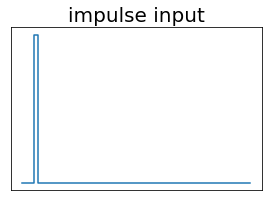
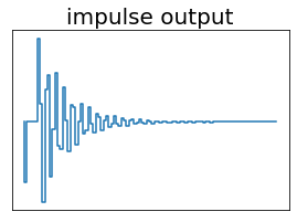
../_images/examples_05_MIMO_Event_19_0.png

[11]:

fig, ax = plt.subplots(figsize=(4.5,3))
ax.step(t, [input(ti) for ti in t], where='post')
ax.set_title('impulse input', fontsize=20)
ax.axes.get_xaxis().set_visible(False)
ax.axes.get_yaxis().set_visible(False)
ax.tick_params(axis='x', labelsize=15)
ax.tick_params(axis='y', labelsize=15)
ax.set_xlabel(r'$t$ (s)', fontsize=20)
ax.set_ylabel(r'$\ddot{u}$ (cm/s$^2$)', fontsize=20);

fig, ax = plt.subplots(figsize=(4.5,3))
ax.step(t, [-k*output[i,0]/m-c*output[i,1]/m-input(i) for i in range(nt)])
ax.set_title('impulse output', fontsize=20)
ax.axes.get_xaxis().set_visible(False)
ax.axes.get_yaxis().set_visible(False)
ax.tick_params(axis='x', labelsize=15)
ax.tick_params(axis='y', labelsize=15)
ax.set_xlabel(r'$t$ (s)', fontsize=20)
ax.set_ylabel(r'$\ddot{u}$ (cm/s$^2$)', fontsize=20);

../_images/examples_05_MIMO_Event_20_0.png

../_images/examples_05_MIMO_Event_20_1.png

[12]:

def husid(accRH, plothusid, dt, lb=0.05, ub=0.95):
    ai = np.tril(np.ones(len(accRH)))@accRH**2
    husid = ai/ai[-1]
    ilb = next(x for x, val in enumerate(husid) if val > lb)
    iub = next(x for x, val in enumerate(husid) if val > ub)
    if plothusid:
        fig, ax = plt.subplots()
        if dt is not None:
            print("duration between ", f"{100*lb}%", " and ", f"{100*ub}%", " (s): ", dt*(iub-ilb))
            ax.plot(dt*np.arange(len(accRH)), husid)
            ax.set_xlabel("time (s)")
        else:
            ax.plot(np.arange(len(accRH)), husid)
            ax.set_xlabel("timestep")
        ax.axhline(husid[ilb], linestyle=":", label=f"{100*lb}%")
        ax.axhline(husid[iub], linestyle="--", label=f"{100*ub}%")
        ax.set_title("Husid Plot")
        ax.legend()
    return (ilb, iub)

[13]:

# San Lorenzo Bent 4 south column base input
from pathlib import Path
import quakeio
event_path = Path("./hayward/58658_003_20210628_18.29.26.P_SanLo.zip")
event = quakeio.read(event_path)
channel = event.match("l", station_channel='25')
response = channel.accel.data
wt = husid(response, False, dt, lb=0.01, ub=0.99)
nt = len(response)
dt = 0.01
nf = dt*nt
t = np.arange(0,nf,dt)
input = lambda t: response[int(t/dt)]

# Mass, stiffness, and damping
m = 1
k = 100
w = np.sqrt(k/m)
c = 0.05*2*m*w

# fig, ax = plt.subplots(1,2, figsize=(15,5))
fig, ax = plt.subplots(1,2, figsize=(20,3))
ax[0].step(t[wt[0]:wt[1]], [input(ti) for ti in t][wt[0]:wt[1]], where='post')
ax[0].set_title('input')
def eom(y,t,m,c,k):
    return [y[1], -k*y[0]/m-c*y[1]/m-input(t)]
output = integrate.odeint(eom, [1e-5,0], t, args=(m,c,k))
accel_output = [-k*output[int(ti/dt),0]/m-c*output[int(ti/dt),1]/m-input(ti) for ti in t]
ax[1].step(t[wt[0]:wt[1]], accel_output[wt[0]:wt[1]], where='post')
# markerline, stemlines, baseline = ax[1].stem(t[wt[0]:wt[1]], accel_output[wt[0]:wt[1]], basefmt=' ', linefmt='-', markerfmt=' ')
# plt.setp(stemlines, 'linewidth', 0.5)
ax[1].set_title('output');
# ax[1].plot(t+pi/3, -0.01*np.sin(w*(t+pi/3)));

# plt.subplots(figsize=(12,3))
# markerline, stemlines, baseline = plt.stem(t[wt[0]:wt[1]], accel_output[wt[0]:wt[1]], basefmt=' ')
# plt.setp(stemlines, 'linewidth', 0.5)
# plt.setp(markerline, 'markersize', 2);

../_images/examples_05_MIMO_Event_22_0.png

[14]:

fig, ax = plt.subplots(figsize=(4.5,3))
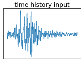
ax.step(t[wt[0]:wt[1]], [input(ti) for ti in t][wt[0]:wt[1]], where='post')
ax.set_title('time history input', fontsize=20)
ax.axes.get_xaxis().set_visible(False)
ax.axes.get_yaxis().set_visible(False)
ax.tick_params(axis='x', labelsize=15)
ax.tick_params(axis='y', labelsize=15)
ax.set_xlabel(r'$t$ (s)', fontsize=20)
ax.set_ylabel(r'$\ddot{u}$ (cm/s$^2$)', fontsize=20);

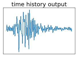
fig, ax = plt.subplots(figsize=(4.5,3))
ax.step(t[wt[0]:wt[1]], accel_output[wt[0]:wt[1]], where='post')
ax.set_title('time history output', fontsize=20)
ax.axes.get_xaxis().set_visible(False)
ax.axes.get_yaxis().set_visible(False)
ax.tick_params(axis='x', labelsize=15)
ax.tick_params(axis='y', labelsize=15)
ax.set_xlabel(r'$t$ (s)', fontsize=20)
ax.set_ylabel(r'$\ddot{u}$ (cm/s$^2$)', fontsize=20);

../_images/examples_05_MIMO_Event_23_0.png

../_images/examples_05_MIMO_Event_23_1.png

Continuous vs Discrete#

\[\dot{x} = A_{c}x\]

\[A_{c} = \Psi \Lambda \Psi^{-1}\]

\[x\left((k+1)\Delta t\right) = A_{d}x(k\Delta t)\]

\[A_{d} = e^{A_{c}\Delta t}\]

\[A_{d} = \Psi \Gamma \Psi^{-1} = e^{\Psi \Lambda \Psi^{-1}\Delta t} = {\Psi e^{\Lambda\Delta t}\Psi^{-1}}\]

\[\Gamma = e^{\Lambda\Delta t}\]

\[\lambda_{j} = \frac{\ln{\gamma_{j}}}{\Delta t}\]

[15]:

import scipy.linalg as sl

dt = 0.01
tf = 10
nt = int(tf/dt)
t = np.arange(0,tf,dt)
assert len(t) == nt

# Mass, stiffness, and damping
m = 1
k = 100
w = np.sqrt(k/m)
c = 0.02*2*m*w
z = c/(2*m*w)

Ac = np.array([[0, 1],[-k/m, -c/m]])
print(f"{Ac=}")
Ad = sl.expm(Ac*dt)
print(f"{Ad=}")

Gam,Psi = sl.eig(Ad)
Lam,Psic = sl.eig(Ac)

print(f"{Psi=}")
print(f"{Psic=}")
print(f"{Gam=}")
print(f"{np.exp(Lam*dt)=}")
print(f"{Lam=}")
print(f"{np.log(Gam)/dt=}")

lams = np.log(Gam)/dt
omegas = np.sqrt(lams*lams.conj())
zetas = -np.real(lams/omegas)
print(f"{omegas=}")
print(f"{zetas=}")
print(f"{w=}")

Ac=array([[   0. ,    1. ],
       [-100. ,   -0.4]])
Ad=array([[ 0.99501082,  0.0099634 ],
       [-0.99634016,  0.99102546]])
Psi=array([[-0.00199007-0.09948382j, -0.00199007+0.09948382j],
       [ 0.99503719+0.j        ,  0.99503719-0.j        ]])
Psic=array([[-0.00199007-0.09948382j, -0.00199007+0.09948382j],
       [ 0.99503719+0.j        ,  0.99503719-0.j        ]])
Gam=array([0.99301814+0.09961409j, 0.99301814-0.09961409j])
np.exp(Lam*dt)=array([0.99301814+0.09961409j, 0.99301814-0.09961409j])
Lam=array([-0.2+9.9979998j, -0.2-9.9979998j])
np.log(Gam)/dt=array([-0.2+9.9979998j, -0.2-9.9979998j])
omegas=array([10.+0.j, 10.+0.j])
zetas=array([0.02, 0.02])
w=10.0

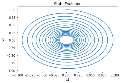
Trajectories#

\[\dot{x} = A_{c}x\]

\[A_{d} = e^{A_{c}\Delta t}\]

\[x\left((k+1)\Delta t\right) = A_{d}x(k\Delta t) = e^{A_{c}\Delta t}x(k\Delta t)\]

[16]:

A1 = np.array([[1,0.1],[-0.1,1]])
A2 = np.array([[0,0.5],[-0.5,0]])
A3 = np.array([[0,1],[-1,-0.5]])

from sympy.matrices import Matrix
display(Matrix(Ac))

$\displaystyle \left[\begin{matrix}0 & 1.0\\-100.0 & -0.4\end{matrix}\right]$

[17]:

x0 = np.array([0,1])
xs = np.zeros((2,nt))
xs[:,0] = x0
for i in range(1,nt):
    # xs[:,i] = A3@xs[:,i-1]
    xs[:,i] = Ad@xs[:,i-1]
    # xs[:,i] = xs[:,i-1]+Ac@xs[:,i-1]*dt

\[x_{k+1} = e^{A_{c}\Delta t}x_{k}\]

[18]:

plt.plot(xs[0], xs[1])
plt.xlabel('x1')
plt.ylabel('x2')
plt.title('State Evolution');

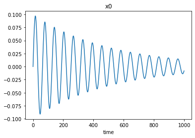
../_images/examples_05_MIMO_Event_30_0.png

[19]:

plt.plot(xs[0])
plt.xlabel('time')
plt.title('x0');

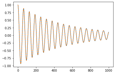
../_images/examples_05_MIMO_Event_31_0.png

[20]:

import sdof
u,v,a = sdof.integrate(m,c,k, np.zeros(nt), dt, v0=1)
plt.plot(v)
plt.plot(xs[1],"--")

[20]:

[<matplotlib.lines.Line2D at 0x20b087f5a00>]

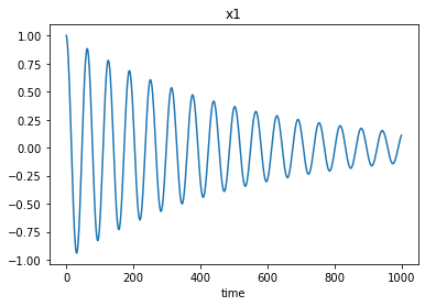
../_images/examples_05_MIMO_Event_32_1.png

[21]:

plt.plot(xs[1])
plt.xlabel('time')
plt.title('x1');

../_images/examples_05_MIMO_Event_33_0.png

ERA#

[22]:

from sympy.matrices import Matrix
from sympy import *
k, m, w, dt, tau = symbols(r'k,m,\omega_{n},{\Delta}t,\tau')
Ac = Matrix(np.array([[0,1],[-w**2,0]]))
Bc = Matrix(np.array([[0],[-1]]))
C = Matrix(np.array([[-w**2,0]]))
D = Matrix(np.array([[-1]]))

display("Ac=", Ac)

'Ac='

$\displaystyle \left[\begin{matrix}0 & 1\\- \omega_{n}^{2} & 0\end{matrix}\right]$

[23]:

display(Ac.diagonalize()[0])

$\displaystyle \left[\begin{matrix}\frac{i}{\omega_{n}} & - \frac{i}{\omega_{n}}\\1 & 1\end{matrix}\right]$

[24]:

display(Ac.diagonalize()[1])

$\displaystyle \left[\begin{matrix}- i \omega_{n} & 0\\0 & i \omega_{n}\end{matrix}\right]$

[25]:

i = np.round((-1)**0.5)
Lam = Matrix(np.array([[i*w, 0],[0,  -i*w]]))
Psi = Matrix(np.array([[1, 1],[i*w, -i*w]]))

[26]:

Psi@Lam@Psi.inv()

[26]:

$\displaystyle \left[\begin{matrix}0 & 1.0\\- 1.0 \omega_{n}^{2} & 0\end{matrix}\right]$

[27]:

A = Psi@exp(Lam*dt)@Psi.inv()

[28]:

A = simplify(exp(Ac*dt))

[29]:

simplify(A)

[29]:

$\displaystyle \left[\begin{matrix}\cos{\left(\omega_{n} {\Delta}t \right)} & \frac{\sin{\left(\omega_{n} {\Delta}t \right)}}{\omega_{n}}\\- \omega_{n} \sin{\left(\omega_{n} {\Delta}t \right)} & \cos{\left(\omega_{n} {\Delta}t \right)}\end{matrix}\right]$

[30]:

Bintegrand = simplify(exp(Ac*tau)@Bc)
Bintegrand

[30]:

$\displaystyle \left[\begin{matrix}- \frac{\sin{\left(\omega_{n} \tau \right)}}{\omega_{n}}\\- \cos{\left(\omega_{n} \tau \right)}\end{matrix}\right]$

[31]:

B = integrate(Bintegrand,(tau,0,dt))
B

[31]:

$\displaystyle \left[\begin{matrix}\begin{cases} \frac{\cos{\left(\omega_{n} {\Delta}t \right)}}{\omega_{n}^{2}} - \frac{1}{\omega_{n}^{2}} & \text{for}\: \omega_{n} > -\infty \wedge \omega_{n} < \infty \wedge \omega_{n} \neq 0 \\0 & \text{otherwise} \end{cases}\\\begin{cases} - \frac{\sin{\left(\omega_{n} {\Delta}t \right)}}{\omega_{n}} & \text{for}\: \omega_{n} > -\infty \wedge \omega_{n} < \infty \wedge \omega_{n} \neq 0 \\- {\Delta}t & \text{otherwise} \end{cases}\end{matrix}\right]$

[32]:

simplify(A.inv()@B)

[32]:

$\displaystyle \left[\begin{matrix}\begin{cases} \frac{1 - \cos{\left(\omega_{n} {\Delta}t \right)}}{\omega_{n}^{2}} & \text{for}\: \omega_{n} > -\infty \wedge \omega_{n} < \infty \wedge \omega_{n} \neq 0 \\\frac{{\Delta}t \sin{\left(\omega_{n} {\Delta}t \right)}}{\omega_{n}} & \text{otherwise} \end{cases}\\\begin{cases} - \frac{\sin{\left(\omega_{n} {\Delta}t \right)}}{\omega_{n}} & \text{for}\: \omega_{n} > -\infty \wedge \omega_{n} < \infty \wedge \omega_{n} \neq 0 \\- {\Delta}t \cos{\left(\omega_{n} {\Delta}t \right)} & \text{otherwise} \end{cases}\end{matrix}\right]$